Drivers of underlying inflation in the euro area over time: a Phillips curve perspective
Published as part of the ECB Economic Bulletin, Issue 4/2019.
In this article we review the evolution of euro area HICP inflation excluding energy and food since the Great Financial Crisis through the lens of the Phillips curve. This period is particularly interesting, as the euro area experienced two recessions (in 2008-2009 and 2011-2014) and a protracted episode of low inflation from 2013 onwards. We estimate a large set of Phillips curve models for the euro area and review the interpretation of inflation developments that they provide over time. We find that our models can account for much of the weakness in underlying inflation between 2013 and mid-2017, but that they cannot account for the weakness in underlying inflation towards the end of our sample.
1 Motivation and overview
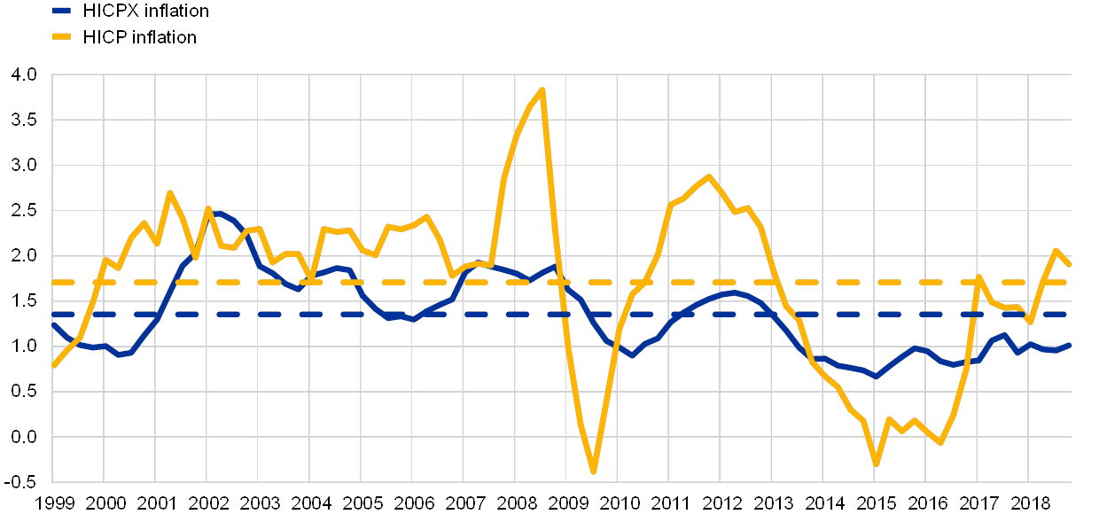
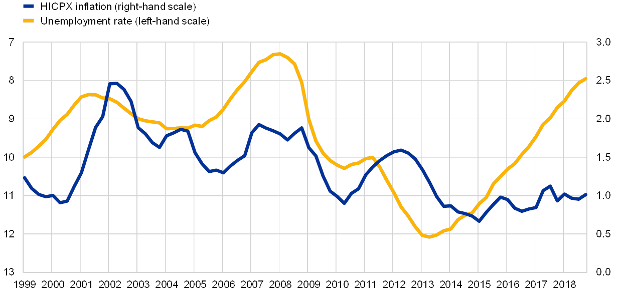
The decade since the onset of the Great Financial Crisis in 2008 is known for a “twin puzzle” in inflation developments across advanced economies. The first years following the crisis are associated with a missing disinflation episode, as inflation appeared to fall by less than the ensuing recessions would have led us to expect.[1] More recently, as most economies gradually recovered, economists have puzzled over missing inflation,[2] with the latter episode being much more prolonged. Taking averages since the launch of the euro as benchmarks, in the euro area both headline HICP inflation and HICP inflation excluding energy and food (HICPX, henceforth “underlying inflation”) dropped below their respective averages after 2009 (see Chart 1), but the missing disinflation view would have predicted an even more marked fall. After a short-lived recovery, inflation rates again fell from 2013 onwards, initiating a protracted period of below-average inflation, which in the case of underlying inflation persists to the present day. The missing inflation view finds the latter episode hard to square with a gradual recovery in economic activity in the euro area that has brought the unemployment rate back to pre-crisis levels (see Chart 2).
Chart 1
HICP inflation and HICP inflation excluding energy and food in the euro area
(annual percentage changes)
Sources: Eurostat and ECB calculations.
Note: The dotted lines represent historical averages since 1999.
Chart 2
HICP inflation excluding energy and food and the unemployment rate in the euro area
(annual percentage changes (right-hand scale), percentages (left-hand scale, inverted))
Source: Eurostat.
Both academics and practitioners use versions of the Phillips curve to understand and communicate inflation developments. In the broadest sense, the Phillips curve is an expression of the notion in economic theory that economic activity, and more precisely the degree of excess demand or supply, should have a bearing on price and inflation developments. The relationship is grounded in many popular economic theories, such as the New Keynesian framework, where inflation is primarily linked to firms’ marginal costs (often proxied with a measure of economic slack) and forward-looking inflation expectations. Phillips curves have long enjoyed great popularity as an empirical tool, but for that very reason the missing disinflation and missing inflation episodes have stirred intense debates about the relationship, including whether it is alive or dead (i.e. steep or flat), and linear or non-linear.
Attempts to simply link the behaviour of inflation to the level of economic activity raise some important questions. For instance, a naïve look at the stability of such a relationship (see Chart 3) would suggest that, compared with the pre-crisis period, the link between real activity and inflation might have “flattened” in the following period, which includes the two puzzling episodes. But many economic factors can shift the level of inflation for a given amount of economic slack, blurring the underlying economic relationship when viewed in a scatterplot. For example, inflation expectations and the cost of imported inputs are important elements of price-setting decisions, and their changes can lead to shifts in the Phillips curve relationship without necessarily changing its slope. On the other hand, the behaviour of economic agents could change over time, for example depending on whether the economy is in recession or not, meaning that the slope could vary over different periods. Without appropriately taking into account such considerations, there is a risk of drawing the wrong conclusions about the strength of the link between inflation and economic activity.
Chart 3
HICPX inflation and the unemployment rate in the euro area
(x-axis: percentages; y-axis: annual percentage changes) Sources: Eurostat and ECB calculations.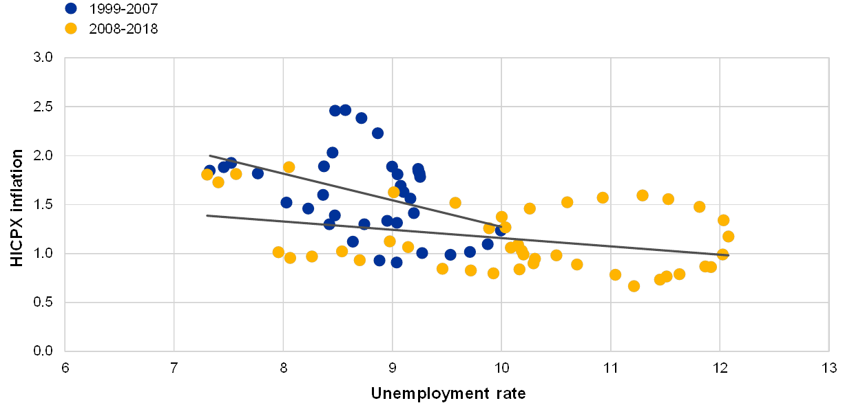
Note: Linear regression lines for the two samples are shown in grey.
The ECB has also relied on Phillips curve models to understand and communicate inflation developments since the Great Financial Crisis. The Phillips curve is an intuitive yet powerful way of conveying the link between inflation and economic activity, which lies at the heart of monetary policy. Thus, as in other central banks and policy institutions (see Box 1 for some case studies), Phillips curves are one element of the analytical toolkit routinely deployed by the ECB to analyse and communicate inflation (and wage growth)[3] developments. Reduced-form estimates of this relationship remain popular due to their simplicity and transparency. However, they require regular review and scrutiny in order to remain useful for analytical, decision-making and communication purposes. This includes all the important choices that have to be made for their empirical set-up: for instance, whether to focus on headline inflation, which is more exposed to commodity prices and other external shocks, or on measures of underlying inflation; what is the most appropriate measure of economic activity to use; what other global and/or domestic drivers of inflation besides economy activity should be included; and whether the relationship should be allowed to change in more complex ways, for example depending on the stage of the economic cycle. Section 2 and Box 2 focus on some of these important issues. In Section 3, we then revisit the recent history of inflation in the euro area through the lens of a large set of reduced-form Phillips curve models, and find that estimated Phillips curves can account for much of the weakness in underlying inflation since 2013, imputing the bulk of it to its key determinants, except for the last few outturns, which cannot be explained well by our models.
Box 1 Other countries’ experiences with Phillips curves
Major central banks use the Phillips curve to assess and communicate inflation developments. For instance, the Federal Reserve System tracks closely how well Phillips curves estimated using a variety of approaches can explain data on the US economy.[4] Some results suggest that in the United States, the link between unemployment and inflation has weakened over time. Indeed, in recent years the United States has been experiencing both low unemployment and low inflation concurrently, which is consistent with a flatter Phillips curve. Federal Reserve Chair Jerome Powell has argued that a number of factors have weakened the effect of labour market tightness on inflation.[5] One factor cited was a more effective conduct of monetary policy, resulting in a stronger anchoring of inflation expectations. Other factors potentially relate to the internationalisation of production structures and the higher import content of goods consumed, which give exchange rates and global prices a greater role in price determination.[6]
A related question, particularly relevant given the very tight labour markets in some advanced economies, including the United States and Japan, is to what extent the Phillips curve is non-linear. In his remarks at the 2019 US Monetary Policy Forum, John Williams also discussed the possibility that the employment-inflation relationship becomes strong only when unemployment is very low, as suggested by Hooper, Mishkin and Sufi (2019).[7] This finding would be highly policy-relevant, as it suggests that while thus far a tight labour market has co-existed with low inflation, a further tightening in the US labour market may lead to inflation rising above target. Williams pointed out that the results for this type of non-linearity in the Phillips curve are often not robust, but their existence would significantly alter the policy trade-offs a central bank is facing.[8]
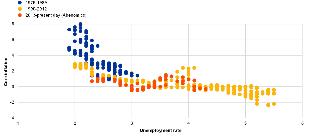
In Japan, the linearity of the Phillips curve has also been questioned.[9] Japan has also been experiencing a tight labour market and low inflation, which could be an indication of a flatter Phillips curve. There are a number of potential explanations for why the country’s low unemployment rate does not feed through more strongly to wage and price inflation. Some factors cited are structural, and relate in part to worker preferences for employment stability over wage increases, as well as hidden labour market slack arising from involuntary part-time workers who are not fully captured by the unemployment rate. However, as in the United States, there is a debate as to when the low and falling unemployment rate should lead to stronger increases in wages and prices. Harada (2018) recently discussed this issue within a Phillips curve framework. He showed estimates suggesting that inflation becomes more responsive to the labour market when the unemployment rate falls below 3%, and concluded that this could imply that the unemployment rate needed to decline further for inflation to reach its target of 2% (see Chart A).[10]
Chart A
Phillips curve for Japan
(x-axis: percentages; y-axis: annual percentage changes)
Sources: Japanese Ministry of Internal Affairs and Communications and Haver Analytics.
Notes: Core inflation in year-on-year percentage changes, measured as the consumer price index for all items excluding fresh food, non-alcoholic beverages, and energy and adjusted for changes in consumption tax. “Abenomics” refers to the economic policies of Japanese Prime Minister Shinzō Abe.
2 Phillips curve models for euro area underlying inflation: what are the choices?
We follow a “thick modelling” approach and bring a large number of reduced-form single-equation Phillips curve models to the data. As emphasised in ECB (2014),[11] there are countless – similarly plausible – empirical specifications of the Phillips curve, reflecting various choices, such as the variables to be included, the functional form and the estimation strategy. One way to mitigate some of this model uncertainty is to choose a generic specification, and estimate different versions of it, changing how we measure each variable – an approach referred to as “thick modelling”.[12] The general specification is the following:
where is inflation, is a measure of inflation expectations, is a measure of economic activity or “slack” and captures external price shocks, which in some specifications are allowed to enter the equation with a longer lag to allow for a slower pass-through to domestic prices. The choice of functional form and estimation strategy addresses tractability and simplicity concerns, but also reflects the proven ability of such models to fit euro area data reasonably well.[13] Effectively, the model is an empirical version of a hybrid New Keynesian Phillips curve, where inflation is driven by forward-looking inflation expectations (proxied here by survey measures), past inflation is allowed to play a role as well (to capture backward-looking expectations and other sources of persistence in price setting) and firms’ marginal costs are proxied by measures of slack or economic activity. External variables are included to control for an important source of supply-side shocks. Figure 1 offers a synopsis of the main specification choices, without aiming to be exhaustive on all possible counts.
Figure 1
Stylised decision tree for the specification of a reduced-form Phillips curve model

Source: ECB.
While the objective of the ECB is unambiguously defined in terms of headline HICP inflation, in this article we focus on measures of underlying inflation, which are less volatile and can help to identify and illustrate the key drivers of price developments (see Figure 1, panel A). Developments in total consumer price index (CPI) inflation may be temporarily influenced by factors that are of a short-term nature, such as swings in commodity prices. In order to focus on the more persistent factors driving inflation, in many empirical applications of the Phillips curve model (and beyond), underlying inflation measures are used instead. However, there are many available measures of underlying inflation. Popular choices include: permanent exclusion measures (such as HICP inflation excluding energy and food), temporary exclusion measures and model-based measures.[14]
We use several measures of economic slack or activity to capture the impact of firms’ costs on inflation (see Figure 1, panel B).[15] Most empirical approaches assume that marginal costs are proportional to economic slack,[16] proxied by the output gap or the unemployment gap. Such unobservable gaps can be obtained by applying statistical filtering techniques, via estimates of potential output based on a production function (e.g. OECD or IMF methodologies), or endogenously, in a manner consistent with inflation developments, as in Blanchard et al. (2015), Jarociński and Lenza (2018) and Chan et al. (2016).[17] Using multiple measures is one way of mitigating the model uncertainty inevitably surrounding estimates of economic slack. Another approach is to directly use observable measures of economic activity, such as the unemployment rate or GDP growth, which, however, has the significant downside of blurring demand and supply factors. More recently, several studies have recommended using the short-term unemployment rate or gap instead of total unemployment measures.[18] Regardless of the reference measure, additional complications arise from estimating slack in real time, partly related to the potentially large revisions to some of the macro data used to proxy slack.[19]
We use available survey measures to proxy inflation expectations (see Figure 1, panel C).[20] The inflation expectations of firms and workers/consumers are not available for most countries, so several strategies have been adopted to address the issue. Backward-looking expectations, i.e. assuming that they are based on past inflation, are the simplest one, and the inclusion of a lagged inflation term in equation (1) is partly motivated by this. To measure forward-looking expectations, survey measures are a convenient way to proxy the beliefs of economic agents regarding future price movements. Their main caveat is that such surveys usually reflect expectations of professional forecasters, which could differ markedly from those of price setters or consumers.[21]
We also control for external supply-side shocks that might hit domestic prices (see Figure 1, panel D).[22] In an increasingly globalised world, both domestic headline and underlying inflation can be sensitive to various external supply-side shocks, such as those coming from commodity and other import prices. There is some empirical evidence for the United States and other countries that import prices do affect inflation in a Phillips curve framework.[23] On the other hand, there is less empirical support when it comes to an independent influence of the global business cycle on domestic inflation.[24]
The relevant variables to include are not the only source of uncertainty in the Phillips curve; the functional form matters as well. The choice of specification is often driven by the scope and purpose of the analysis; for example, if a linear specification turns out not to offer a satisfactory explanation of outcomes, non-linear specifications can be deployed. Box 2 discusses some important departures from the linear benchmark model in equation (1) in the context of recent ECB work on Phillips curves.
We estimate 550 versions of the baseline model and find the euro area Phillips curve to be alive, but we also find evidence pointing to the importance of inflation drivers other than domestic real activity. Estimation results point to a statistically significant and economically plausible link between euro area inflation and its key drivers. Focusing on the relationship with real activity, Chart 4 shows the Phillips curve slope across specifications for each measure of slack or economic activity. In virtually all 550 models under review, the real activity measure is statistically significant with the theoretically implied sign, confirming the visual impression given in Chart 2 regarding the co-movement between underlying inflation and economic activity in the euro area. However, the slope is generally not very steep and the coefficients of other relevant drivers, such as inertia, expectations and external shocks, are often also significant, pointing to the importance of factors beyond slack for adequately explaining inflation developments. In other words, not only movements along the Phillips curve, but also shifts in the curve, need to be taken into account.
Chart 4
Estimated Phillips curve slope across all specifications
(regression coefficients on standardised measures of economic slack/tightness)

Sources: European Commission, ECB, Eurostat, IMF, OECD and ECB calculations.
Notes: We consider the following measures of slack: (1) output gap – model-based estimate; (2) output gap – IMF; (3) output gap – European Commission; (4) output gap – OECD; (5) unemployment rate; (6) unemployment gap – model-based estimate; (7) unemployment gap – IMF; (8) unemployment gap – European Commission; (9) unemployment gap – OECD; (10) short-term unemployment rate; (11) the U6 measure. The unemployment rates/gaps have been inverted. Sample: Q1 1995 to Q3 2018. All measures of slack/tightness are standardised for the coefficients to be comparable across specifications. The vertical bars show the range of coefficients across all specifications including a particular measure of economic slack/tightness or activity.
Box 2 Linear and non-linear Phillips curves
Empirical Phillips curve models are often linear. Equation (1) in Section 2 is a fairly standard specification of a single-equation linear Phillips curve, where lagged inflation, a measure of slack, a measure of inflation expectations and a measure of import prices are included. Linearity refers both to linearity of the parameters (the right-hand-side term is a linear function) and of the variables (i.e. variables enter the equation with the units they are measured in). Both assumptions can be relaxed in a number of ways.
There are several possible non-linear specifications of the Phillips curve. The most common forms of non-linearity include transformations of the independent variables, such as square (or even higher-order) slack terms, which can introduce both convexity and concavity in Phillips curves. Similar and more sophisticated relationships can be fitted by weighting the slack measure with another variable that captures the state of the economy; for example, a simple dummy variable can achieve several forms of “piecewise linearity”, which can approximate different regimes, such as booms and deep recessions, as opposed to “normal times”. More sophisticated devices, such as non-linear splines or Markov switching, are sometimes also used in the estimation of non-linear Phillips curves.[25]
Behind the notion of a non-linear Phillips curve often lies the idea that pricing behaviour could be different at different stages of the economic cycle. This in turn might be due to psychological, institutional or technological considerations and their interplay in a modern market economy. One argument with a long history relates to downward nominal wage rigidities; i.e. workers being reluctant to accept (or firms to impose) cuts in nominal wages in a downturn. This could be due to collective bargaining arrangements, or a psychological reluctance to see one’s pay cut in nominal terms. The implication is that in the presence of a large amount of economic slack, wages (and therefore prices) will change at a different rate than during more normal periods, thus potentially bending the Phillips curve into a more convex shape. A similar phenomenon can occur if firms experience short-run capacity constraints that make it difficult to immediately satisfy further increases in demand. One example would be mothballed equipment that can only be put back into use with a time lag and at some cost. In such a situation, firms might increase prices before increasing their capacity to fully satisfy the additional demand, whereas in more normal times they would adjust inputs to production first, thus again making the Phillips curve more convex. Another source of convexity is the idea that price changes could be more frequent in periods of high inflation.
Some theories predict a concave rather than a convex Phillips curve, i.e. inflation being more responsive to slack when there is a large amount of it than in normal times or booms. For example, this is consistent with firms operating in market structures where they can make different pricing decisions depending on market conditions. When there is a large amount of slack, firms may be more willing to cut prices in order not to lose market share to rival firms. Conversely, firms might be reluctant to increase prices in periods when output is close to or above potential to avoid losing market share.
Convexity and concavity do not need to be mutually exclusive. One way to reconcile the presence of both are “threshold effects”, namely a steeper relationship between inflation and slack only for extreme values of the slack variable (e.g. during deep recessions and/or after prolonged periods of above-trend growth). One microeconomic notion consistent with such a set-up is that prices are more responsive when there is a lot of slack (because firms do not want to lose market share) or when firms are operating way above potential (because of higher costs), and less responsive in between (when adjusting factor utilisation is preferred to changing prices). In such a case, the Phillips curve is concave when there is a lot of slack and convex when the economy is operating considerably above potential.
Other microeconomic arguments for non-linearity do not fit the convexity-concavity dichotomy as neatly, but may nonetheless be important. This may either be because they only operate during upturns or downturns, or because they depend on the rate at which slack is closing. Menu costs are one example: when firms face costs to change their prices, typically only a fraction of them will adjust prices in a given period, but it is likely that the larger the demand shock they face, the greater the share of firms adjusting their prices will be. In such a case, the rate at which slack closes (or opens up) will determine the slope of the Phillips curve for any given level of slack.
Chart B
Euro area Phillips curve slopes in two samples across a range of specifications
(regression coefficients on standardised measures of economic slack/tightness)
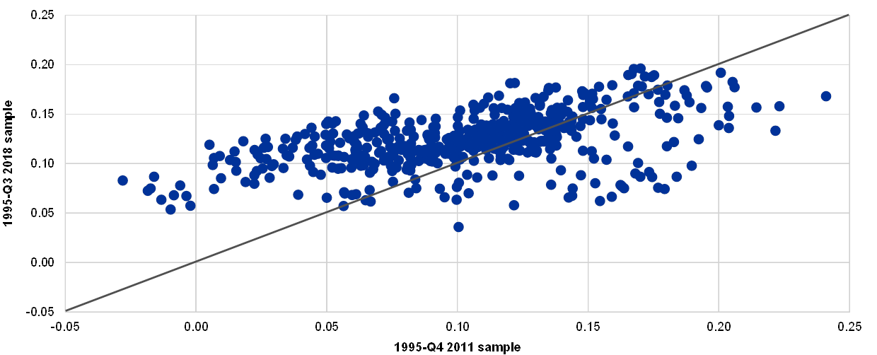
Sources: European Commission, ECB, Eurostat, IMF, OECD and ECB calculations.
Note: Slack measures are as in Chart 4, standardised (and inverted where appropriate) for comparability.
Time variation in the coefficients of an otherwise linear Phillips curve is sometimes taken as first-pass evidence of non-linearity in the relationship between slack and inflation. That is because, if the pattern of variation coincides with the economic cycle, then time-varying parameters might be a better fit for outturns that would otherwise look non-linear when viewed in slack/inflation space. Time variation in the coefficients is in itself a form of non-linearity, because the parameters in the equation effectively become variables that depend on time and multiply the independent variables. Broadly speaking, time variation has been tested in two ways: either by simply splitting the sample and comparing fixed parameter estimates, or by estimating models with time-varying parameters. Both approaches provide some evidence of an increase in the slope of the euro area Phillips curve in recent years, although with a high degree of uncertainty. Chart B illustrates the results from the first approach: the same models are estimated over two different samples, and changes in slope across the two samples are illustrated by means of deviations from a 45 degree line.
Quadratic slack terms and other forms of non-linearity have been tested extensively, with mixed results. In an empirical exercise featuring a large number of different specifications, quadratic slack terms (which seek to introduce convexity in the relationship between slack and inflation) were statistically significant in some of the specifications, but, in models that controlled for imported inflation, that significance largely disappeared, consistent with the view that linear models with suitably chosen control variables are even able to fit data well that appear non-linear in a reduced-form relationship (see Chart C). In the same exercise, a dummy variable for positive values of the output gap (in principle able to fit both convex and concave relationships) turned out to be significant only in a fraction of the models.
Chart C
Share of instances in which the non-linear variables in euro area Phillips curve specifications are statistically significant
(percentages) Sources: Eurostat and ECB staff calculations.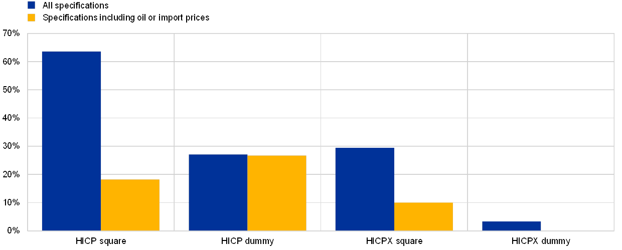
Notes: For two measures of inflation (HICP and HICPX inflation), versions of equation (1) including and excluding external variables and a different form of non-linearity (quadratic terms for economic slack or 0/1 dummy variables for economic slack above/below a certain threshold) are estimated for various measures of slack (see the notes to Chart 4). The bars denote the share of models in which the coefficients on the non-linear terms are statistically significant at the 10% level.
Some evidence in favour of non-linearity comes from considering more sophisticated threshold effects. Models allowing for a steeper slope of the Phillips curve when slack is outside certain bounds help fit the data even when including expectations and imported inflation in the specification. This is the case both when the output gap and when the unemployment gap are used as measures of slack. Using regime-switching Phillips curves, where the slope is allowed to change with the level of the output gap, some evidence of non-linearity was found for the euro area.[26]
3 The drivers of euro area underlying inflation implied by Phillips curve models
Phillips curve models can provide a historical perspective on the relative importance of the main drivers of underlying inflation. Chart 5 summarises the lessons that can be drawn from the thick modelling approach presented in the previous section by showing the average contributions to inflation (all in terms of deviations from their historical averages) of its three main drivers across all models considered.[27] At the onset of the Great Financial Crisis, underlying inflation was well above its historical average, largely explained by the economy running at above normal capacity (see the large contributions from economic tightness). However, as early as the second half of 2009, the inflation gap – the deviation of inflation from its mean – turned negative. To a certain extent, this was due to increasing levels of slack with the unfolding of the ensuing recession, and also to a slight softening of inflation expectations, but part of the weakness cannot be accounted for by our explanatory variables.
Chart 5
Phillips curve-based decomposition of underlying inflation
(annual percentage changes and percentage point contributions; all values in terms of deviations from their averages since 1999)
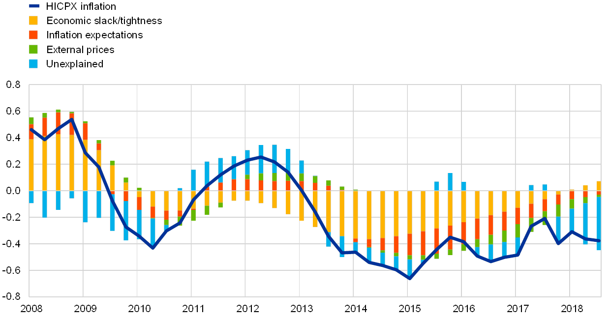
Source: ECB calculations.
Notes: The bars show average contributions across all the models considered in Section 2. Contributions are derived as in Yellen, J.L., “Inflation Dynamics and Monetary Policy”, speech at the Philip Gamble Memorial Lecture, University of Massachusetts, Amherst, 24 September 2015.
The missing disinflation and missing inflation episodes are partly reflected in Phillips curve estimates. The evidence presented in Chart 5 supports the missing disinflation narrative from 2011 onwards, when a large unexplained positive contribution to underlying inflation begins to appear. One explanation put forward for this pointed to a larger impact from external factors during the recovery phase than simple Phillips curve models could capture.[28] In the course of 2013, underlying inflation fell well below its historical average, where it has remained until the present day. The Phillips curve models lend some support to this missing inflation puzzle, as the negative contributions from the residuals indicate the models’ inability to fully account for the weakness in inflation over almost the entire period. One explanation is related to “pent-up restraints”: while declines in prices and wages during the recession were limited due to downward nominal rigidities, in the early phases of the recovery, price and wage inflation may have been correspondingly subdued.[29] In other words, the missing inflation could have been a consequence of the missing disinflation period, at least in the initial stages of the economic recovery.
Nevertheless, except for the last year or so, estimated Phillips curves can account for much of the weakness in underlying inflation since 2013, imputing the bulk of it to its key determinants rather than to unexplained residuals. The relative importance of the three key inflation drivers has changed throughout this period. Based on the average contributions across models in Chart 5, the drag coming from economic slack dominated the picture in the early part of the period, and continued to play a (diminishing) role until spare capacity in the euro area was largely absorbed. As underlying inflation continued to turn out well below its historical average, some of its weakness began being attributed to lower short-to-medium-term inflation expectations, which exerted a mild drag up to recent quarters. External developments, in the form of lower oil, commodity and other import prices, also began gradually to feed through to underlying inflation. While the negative contributions of these factors had largely faded by early 2018, underlying inflation remained weak throughout 2018.
The more recent weakness in underlying inflation is difficult to explain within the Phillips curve framework. Even within our thick modelling framework, the narrative summarised in Chart 5 is subject to a large degree of uncertainty, as different models impute inflation developments to different factors at any given point in time. In the following subsections, we provide a quantification of the uncertainty around the contributions of slack, inflation expectations and external prices to inflation, and also review some of the economic sources of such uncertainty. The overall picture that emerges is that uncertainty surrounding individual drivers could potentially account for some of the unexplained residuals in Chart 5 until mid-2017, but given the fading contributions of all three main drivers, the more recent weakness in underlying inflation cannot be accounted for by standard Phillips curve models.
Slack
Slack played a leading role in explaining underlying inflation from 2013 until 2016. Given the euro area sovereign debt crisis in 2010 and the ensuing recession (2011-2014), it is understandable that explanations of inflation over that period focus on the role of domestic drivers, especially slack, in the euro area.[30] Nevertheless, Phillips curve models do not paint the full picture; the initial fall in underlying inflation after mid-2012 was unexpected, and although slack can account for the bulk of it in Chart 5, unexplained factors also played a major role.[31] Furthermore, the range of contributions of slack to inflation across the 550 models that we estimate is particularly wide over that period (see Chart 6). Two explanations for the difficulty in explaining inflation over that period using simple Phillips curve models are a steepening of the euro area Phillips curve (whereby inflation would follow the business cycle much more closely) and/or a mismeasurement of slack (namely more slack than captured by standard measures).
Chart 6
Range of contributions of slack to underlying inflation
(annual percentage changes and percentage point contributions; all values in terms of deviations from their averages since 1999)
Source: ECB calculations.
Notes: The shaded area shows the range of contributions of measures of economic slack/tightness to underlying inflation across the 550 models that we estimate (see Section 2); the broken grey line shows the average contribution, which corresponds to the yellow bars in Chart 5. Contributions are derived as in Yellen, J.L., “Inflation Dynamics and Monetary Policy”, speech at the Philip Gamble Memorial Lecture, University of Massachusetts, Amherst, 24 September 2015.
Changes in Phillips curve slopes and potential mismeasurement of slack add to the uncertainty surrounding the contribution of slack to inflation. As early as 2014,[32] the ECB discussed the possibility of a stronger relationship between inflation and slack, and lower nominal rigidities in some euro area countries due to structural reforms[33] being implemented are consistent with such a view. Nevertheless, it is challenging to distinguish a change in the Phillips curve slope from a mismeasurement of slack. Alternative estimates of slack, where the output gap is required to be consistent with inflation dynamics within a stable Phillips curve relationship, would have to have been much larger over the missing inflation period.[34] Also, the legacy of the prolonged euro area sovereign debt crisis suggested that the full extent of slack in the labour market could be better captured by broadening the range of labour market indicators, also taking into account workers who became discouraged or worked part-time for economic reasons, but Phillips curves estimated with such measures would still show negative residuals in the more recent period.[35] Moreover, real-time estimates of economic slack can be subject to large measurement error, and revisions are common.[36] Notwithstanding all these sources of uncertainty, Chart 6 suggests that, over the most recent period, the drag from slack has dissipated, making it difficult to look to this factor to account for the unexplained negative residuals in Chart 5 in the last year of the sample.
Inflation expectations
The decline in survey-based measures of inflation expectations after 2013 raised some concerns that the Phillips curve had shifted downwards, but the message from our estimates is mixed. Over the period from 2014 to mid-2017, Chart 5 shows that inflation expectations might have contributed to the drag on underlying inflation. Nevertheless, as discussed in Section 2, available measures of expectations are imperfect and it is sometimes difficult to interpret the signal they provide for inflation. Chart 7 highlights this uncertainty within our thick modelling framework. The range of the contributions of expectations over the 2014-2017 period can be wide at times, reflecting the fact that it covers measures with various forecast horizons, including both short-to-medium-term survey-based inflation expectations (which can be noisier and more closely trail developments in past inflation) and long-term measures of survey inflation expectations (which, by comparison, have been more stable).
The most recent weakness in underlying inflation does not appear to be explained by developments in inflation expectations. Not only has the average contribution gradually faded towards zero, but the range of contributions across models has also become remarkably small, reflecting the gradual pick-up in the available survey-based measures of inflation expectations.
Chart 7
Range of contributions of inflation expectations to underlying inflation
(annual percentage changes and percentage point contributions; all values in terms of deviations from their averages since 1999)
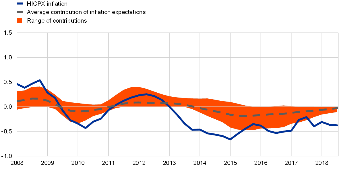
Source: ECB calculations.
Notes: The shaded area shows the range of contributions of measures of inflation expectations to underlying inflation across the 550 models that we estimate (see Section 2); the broken grey line shows the average contribution, which corresponds to the red bars in Chart 5. Contributions are derived as in Yellen, J.L., “Inflation Dynamics and Monetary Policy”, speech at the Philip Gamble Memorial Lecture, University of Massachusetts, Amherst, 24 September 2015.
External factors
Global factors in general, and low oil and other commodity prices in particular, have featured prominently in inflation narratives over recent years.[37] Chart 5 highlights the increasing drag on underlying inflation associated with external price developments from 2015 onwards. Underlying inflation is affected by external price movements through two main channels: a direct one, via the price of imported final consumption goods; and an indirect one, via the price of imported intermediate goods used in production within the euro area. The drop in oil prices starting in mid-2014 was one of the largest since the inception of Economic and Monetary Union (EMU) and left its mark on the headline inflation profile for the subsequent years. For underlying inflation, however, the negative contributions from external price developments were relatively modest when looking at the average contribution across models, but for part of this period could have been substantially larger, according to our range of estimates (see Chart 8). However, over the last few quarters, both the average contribution and the range around it have shrunk substantially.
Chart 8
Range of contributions of external prices to underlying inflation
(annual percentage changes and percentage point contributions; all values in terms of deviations from their averages since 1999)

Source: ECB calculations.
Notes: The shaded area shows the range of contributions of measures of external prices to underlying inflation across the 550 models that we estimate (see Section 2); the broken grey line shows the average contribution, which corresponds to the green bars in Chart 5. Contributions are derived as in Yellen, J.L., “Inflation Dynamics and Monetary Policy”, speech at the Philip Gamble Memorial Lecture, University of Massachusetts, Amherst, 24 September 2015.
Global influences on domestic inflation could extend beyond what can be captured by import and commodity prices alone, but the empirical evidence on additional channels is mixed. In a globalising world, the inflation process might reflect increased trade flows, the integration of emerging economies into the world economy and the rise of global value chains shifting parts of production abroad. All these phenomena can affect inflation via numerous channels, potentially with long lags, and capturing their influence within a traditional Phillips curve model can be empirically challenging. ECB (2017) finds some support for including global measures of slack in a thick modelling Phillips curve framework, but overall the explanatory gains appear to be limited.[38] However, despite the mixed empirical results, the relatively low dispersion of inflation rates across different economies, including in the case of underlying inflation (see Chart 9), suggests that broader structural drivers may be shaping inflation worldwide in ways that are yet to be fully grasped.[39]
Chart 9
Dispersion of underlying inflation rates in OECD countries since 1999
(standard deviations)

Sources: Haver Analytics, ECB and Eurostat.
Note: The line shows the standard deviation across OECD countries excluding Turkey and Slovenia.
4 Conclusions
Phillips curve models provide a useful and intuitive framework for understanding and communicating inflation developments. We employ a parsimonious, yet not overly simplistic specification that spans the key determinants of inflation beyond the level of economic activity. We combine it with a thick modelling approach that mitigates some of the pervasive model uncertainty, allowing us to draw a more robust inference about the strength of the relationship between inflation and its drivers. Our results provide a plausible narrative for the evolution of underlying inflation in the euro area since the onset of the Great Financial Crisis.
Estimated Phillips curves can account for much of the weakness in underlying inflation between 2013 and mid-2017, while the more recent weakness in underlying inflation remains largely unexplained. The average contributions of slack, inflation expectations and external prices across all estimated models can account for the bulk of the deviations of underlying inflation from its historical average over large spans of the period we consider. However, given the fading contributions of all three factors and the narrowing of uncertainty ranges around them over the most recent period, the persistent weakness in underlying inflation highlights the need for other, complementary, approaches.
Like any other analytical tool, Phillips curves also have limitations and shortcomings. For example, while being intuitive and transparent, reduced-form estimates are, by nature, partial-equilibrium and thus open to both theoretical and empirical objections. Furthermore, to remain tractable, they inevitably miss many aspects (for example, fiscal policy and financial factors) that could nonetheless be important for explaining underlying inflation but require more sophisticated modelling approaches. Finally, statistical and measurement issues can also cause instability in Phillips curve relationships over specific periods of time. Despite these shortcomings, Phillips curve models are an integral part of a much broader analytical toolkit deployed by central banks to understand the inflation process. They have often provided relevant insights, at times leading the way for more sophisticated approaches and at other times offering a cross-check for analyses or forecasts originating elsewhere. The very lively debate surrounding them bears testimony to their usefulness.
- Coibion, O. and Gorodnichenko, Y., “Is the Phillips Curve Alive and Well after All? Inflation Expectations and the Missing Disinflation”, American Economic Journal: Macroeconomics, Vol. 7(1), 2015, pp. 197-232; Ciccarelli, M. and Osbat, C. (eds.), “Low inflation in the euro area: Causes and consequences”, Occasional Paper Series, No 181, ECB, 2017.
- Constâncio, V., “Understanding Inflation Dynamics and Monetary Policy”, panel remarks at the Jackson Hole Economic Policy Symposium, Federal Reserve Bank of Kansas City, 29 August 2015; Bobeica, E. and Jarociński, M., “Missing Disinflation and Missing Inflation: A VAR Perspective”, International Journal of Central Banking, Vol. 15(1), 2019, pp. 199-232.
- See Box 3 in the article entitled “The euro area labour market through the lens of the Beveridge curve” in this issue of the Economic Bulletin.
- See Yellen, J.L., “Inflation Dynamics and Monetary Policy”, speech at the Philip Gamble Memorial Lecture, University of Massachusetts, Amherst, 24 September 2015. Yellen, J.L., “Inflation, Uncertainty and Monetary Policy”, speech at the 59th Annual Meeting of the National Association for Business Economics, Cleveland, Ohio, 26 September 2017.
- Powell, J., “Monetary Policy and Risk Management at a Time of Low Inflation and Low Unemployment”, speech at the 60th Annual Meeting of the National Association for Business Economics, 2 October 2018.
- Williams, J.C., “Discussion of ‘Prospects for Inflation in a High Pressure Economy: Is the Phillips Curve Dead or Is It Just Hibernating?’ by Peter Hooper, Frederic S. Mishkin, and Amir Sufi”, remarks at the 2019 US Monetary Policy Forum, Federal Reserve Bank of New York, 22 February 2019.
- Williams (2019), op. cit.; and Hooper, P., Mishkin, F.S. and Sufi, A., “Prospects for Inflation in a High Pressure Economy: Is the Phillips Curve Dead or is It Just Hibernating?”, paper presented at the 2019 US Monetary Policy Forum, February 2019. For a theoretical derivation of a non-linear Phillips curve, see Benigno, P. and Ricci, L., “The Inflation-Output Trade-Off with Downward Wage Rigidities”, American Economic Review, Vol. 101(4), 2011, pp. 1436-1466; for an empirical review of the evidence, see, e.g., Albuquerque, B. and Baumann, U., “Will US inflation awake from the dead? The role of slack and non-linearities in the Phillips curve”, Journal of Policy Modeling, Vol. 39(2), 2017, pp. 247-271.
- This result, and the accompanying caveat, parallels some of the findings on the potential non-linearity of the Phillips curve relationship in the euro area discussed in Box 2.
- See, for example, Iwasaki, Y., Muto, I. and Shintani, M., “Missing Wage Inflation? Downward Wage Rigidity and the Natural Rate of Unemployment”, Bank of Japan Research Laboratory Series, No 18-E-3, 2018; Hara, N., Kazuhiro, H. and Ichise, Y., “Changing Exchange Rate Pass-Through in Japan: Does It Indicate Changing Pricing Behavior?”, Bank of Japan Working Paper Series, No 15-E-4, 2015.
- Harada, Y., “Economic Activity, Prices and Monetary Policy in Japan,” speech, Ishikawa, Japan, 4 July 2018.
- “The Phillips curve relationship in the euro area”, Monthly Bulletin, ECB, July 2014.
- Granger, C.W.J. and Jeon, Y., “Thick modeling”, Economic Modelling, Vol. 21(2), 2004, pp. 323-343.
- For a discussion of this specification, see Ciccarelli and Osbat, eds. (2017), op. cit. Phillips curve relationships are also part of richer structural models; in this article we focus on reduced-form evidence, mainly for the sake of simplicity of exposition.
- All three types of measure are explained and discussed in Ehrmann, M., Ferrucci, G., Lenza, M. and O’Brien, D., “Measures of underlying inflation for the euro area”, Economic Bulletin, Issue 4, ECB, 2018.
- See the notes to Chart 4 for the list of measures of slack considered.
- One exception, where instead the labour share of income is used as a measure of real marginal costs, is Galí, J. and Gertler, M., “Inflation dynamics: A structural econometric analysis”, Journal of Monetary Economics, Vol. 44(2), 1999, pp. 195-222.
- Blanchard, O., Cerutti, E. and Summers, L.H., “Inflation and Activity: Two Explorations and Their Monetary Policy Implications”, Working Paper Series, No WP 15-19, Peterson Institute for International Economics, 2015; Jarociński, M. and Lenza, M., “An Inflation-Predicting Measure of the Output Gap in the Euro Area”, Journal of Money, Credit and Banking, Vol. 50(6), 2018, pp. 1189-1224; Chan, J.C.C., Koop, G. and Potter, S.M., “A Bounded Model of Time Variation in Trend Inflation, Nairu and the Phillips Curve”, Journal of Applied Econometrics, Vol. 31(3), 2016, pp. 551-565.
- See Ball, L. and Mazumder, S., “A Phillips Curve with Anchored Expectations and Short-Term Unemployment”, Journal of Money, Credit and Banking, Vol. 51(1), 2019, pp. 111-137, and the references therein.
- See Szörfi, B. and Tóth, M., “Measures of slack in the euro area”, Economic Bulletin, Issue 3, ECB, 2018.
- We consider the following inflation expectation measures: (1-7) Consensus Economics measures with a horizon of two to seven quarters ahead and interpolated long-term Consensus Economics expectations; (8-11) ECB Survey of Professional Forecasters measures, one year ahead, two years ahead and five years ahead.
- Coibion and Gorodnichenko (2015), op. cit., point to the difference between the inflation expectations of professional forecasters and of firms, arguing that the latter are better approximated by the expectations of consumers.
- As external variables, we employ: (1) annual change in the prices of imports from outside the euro area; (2) annual change in oil prices in euro; (3) a longer-term average of past oil price changes; (4-5) annual global headline and underlying inflation, all with appropriately long lags.
- Matheson, T. and Stavrev, E., “The Great Recession and the inflation puzzle”, Economics Letters, Vol. 120(3), 2013, pp. 468-472; Forbes, K.J., “How Have Shanghai, Saudi Arabia, and Supply Chains Affected U.S. Inflation Dynamics?”, Federal Reserve Bank of St. Louis Review, Vol. 101(1), First Quarter 2019, pp. 27-43.
- “Domestic and global drivers of inflation in the euro area”, Economic Bulletin, Issue 4, ECB, 2017.
- See, for example, Leduc, S., Marti, C. and Wilson, D.J., “Does Ultra-Low Unemployment Spur Rapid Wage Growth?”, FRBSF Economic Letter, No 2019-02, Federal Reserve Bank of San Francisco, 2019.
- Gross, M. and Semmler, W., “Mind the output gap: the disconnect of growth and inflation during recessions and convex Phillips curves in the euro area”, Working Paper Series, No 2004, ECB, 2017.
- This is an ex post analysis involving the full sample, but a real-time one would have painted a similar picture for the low-inflation period.
- Constâncio (2015), op. cit.; Ciccarelli and Osbat, eds. (2017), op. cit.; and Bobeica and Jarociński (2019), op. cit. Increases in VAT in some euro area countries over the period could also account for part of this unexplained contribution, but only to a limited extent.
- Praet, P., “Price stability: a sinking will-o’-the-wisp?”, IMF Spring Meetings Seminar, Washington, D.C., 16 April 2015.
- Ciccarelli and Osbat, eds. (2017), op. cit.
- This is a point about changes in, rather than the level of, inflation: the main contributor to the peak-to-trough fall in inflation is the change in the contribution from the residual rather than that from slack.
- ECB (2014), op. cit.
- Izquierdo, M., Jimeno, J.F., Kosma, T., Lamo, A., Millard, S., Rõõm, T. and Viviano, E., “Labour market adjustment in Europe during the crisis: microeconomic evidence from the Wage Dynamics Network survey”, Occasional Paper Series, No 192, ECB, June 2017.
- Jarociński and Lenza (2018), op. cit.
- Cœuré, B., “Scars or scratches? Hysteresis in the euro area”, speech at the International Center for Monetary and Banking Studies, Geneva, 19 May 2017. This argument is one of the reasons for including broad unemployment measures in our estimates (see the notes to Chart 4).
- See Szörfi and Tóth (2018), op. cit.
- For example, “External environment”, Economic Bulletin, Issue 8, ECB, 2015, noted that “global inflation has remained very low, reflecting the fall in oil prices”.
- See “Domestic and global drivers of inflation in the euro area”, Economic Bulletin, Issue 4, ECB, 2017; and Nickel, C., “The role of foreign slack in domestic inflation in the Eurozone”, VOX, CEPR Policy Portal, 28 July 2017.
- See also Forbes (2019), op. cit.


